Zooming Through Euler Path: Supercharging with GPU

So, continuing where we left off:

1. Walking the Euler Path: Intro
2. Visualizing Graphs
3. Walking the Euler Path: GPU for the Road
4. Walking the Euler Path: PIN Cracking and DNA Sequencing

For the Win

And finally I ran the GPU-enabled algorithm for finding the Euler path.

let sw = Stopwatch()
let N = 1024 * 1024
let k = 7
let avgedges k = [1..k] |> List.map float |> List.average
let gr = StrGraph.GenerateEulerGraph(N * 10, k)
printfn "Generated euler graph in %A, edges: %s" sw.Elapsed (String.Format("{0:N0}", gr.NumEdges))

let eulerCycle = findEulerTimed gr // GPU-based algorithm
sw.Restart()
let eulerVert = gr.FindEulerCycle() // Hierholzer algorithm
sw.Stop()
let cpu = float sw.ElapsedMilliseconds
printfn "CPU: Euler cycle generated in %A" sw.Elapsed

And the results:

Generating euler graph: vertices = 10,485,760; avg out/vertex: 4
Generated euler graph in 00:00:19.7520656, edges: 41,944,529
Euler graph: vertices - 10,485,760.00, edges - 41,944,529.00
1. Predecessors computed in 00:00:03.2146705
2. Partitioned linear graph in 00:00:06.4475982
Partitions of LG: 6
3. Circuit graph generated in 00:00:31.4655218
4. Swips implemented in 00:00:00.2189634

GPU: Euler cycle generated in 00:00:41.3474044
CPU: Euler cycle generated in 00:01:02.9022833

And I was like: WOW! Finally! Victory is mine! This is awesome! I’m awesome, etc. Victory dance, expensive cognac.
Then, after the euphoria subsided a little, I decided to make the mandatory chart:

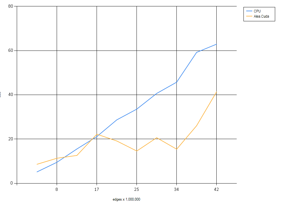
Well, this was sobering!
While the CPU series line displays expected behavior, something is definitely not right with the GPU series: there is obviously some variable at work that I am not taking into account. So, from the beginning.

The Algorithm

I owe the algorithm to this master thesis, which actually implements the algorithm proposed by B. Awerbuch, A. Israeli and Y. Shiloach, “Finding euler circuits in logarithmic parallel time,” in Proceedings of the Sixteenth Annual ACM Symposium on Theory of Computing, 1984, pp. 249-257.

The algorithm as I see it may be split into 4 stages (even 3, but 4 is slightly more convenient implementation-wise). Let’s illustrate.
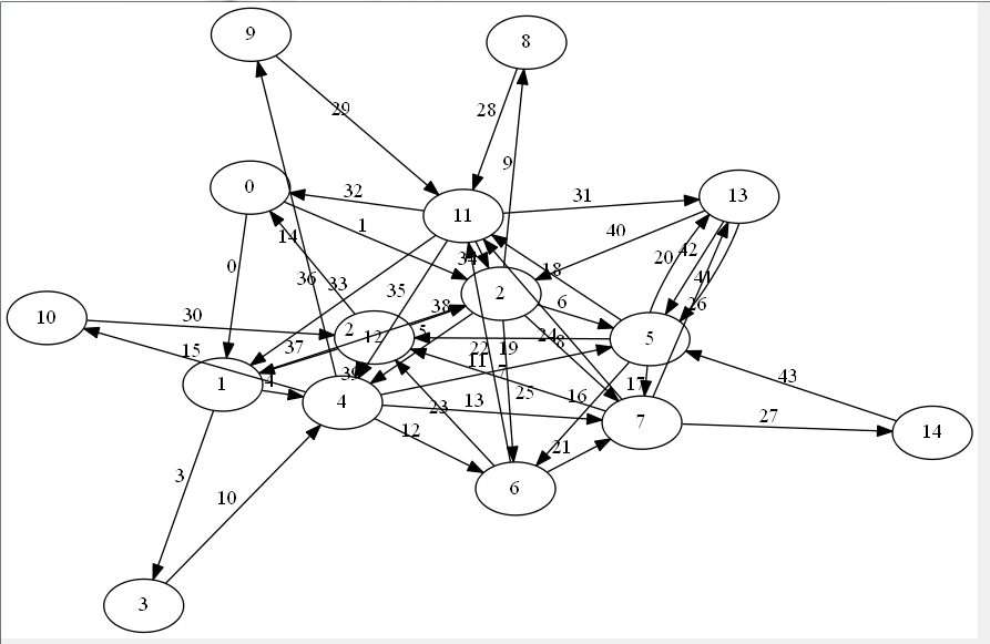
Start with an Euler graph like the one below. It has 15 vertices with an average of 3 edges/vertex in one direction (maxOutOrInEdges = k, we have 44 edges in this case):

let N = 15
let k = 5
let gr = StrGraph.GenerateEulerGraph(N, k)
gr.Visualize(edges=true)

1. We walk it as we like, computing edge predecessors. For two edges is a predecessor of iff , i.e. One edge begins where its predecessor ends. In our representation it’s easy to construct the array of predecessors:

let predecessors (gr : DirectedGraph<'a>) =

    let rowIndex = arrayCopy gr.RowIndex
    let ends = gr.ColIndex

    let predecessors = Array.create gr.NumEdges -1

    [|0..ends.Length - 1|]
        |> Array.iter
        (fun i ->
            predecessors.[rowIndex.[ends.[i]]] <- i
            rowIndex.[ends.[i]] <- rowIndex.[ends.[i]] + 1
        )

    predecessors

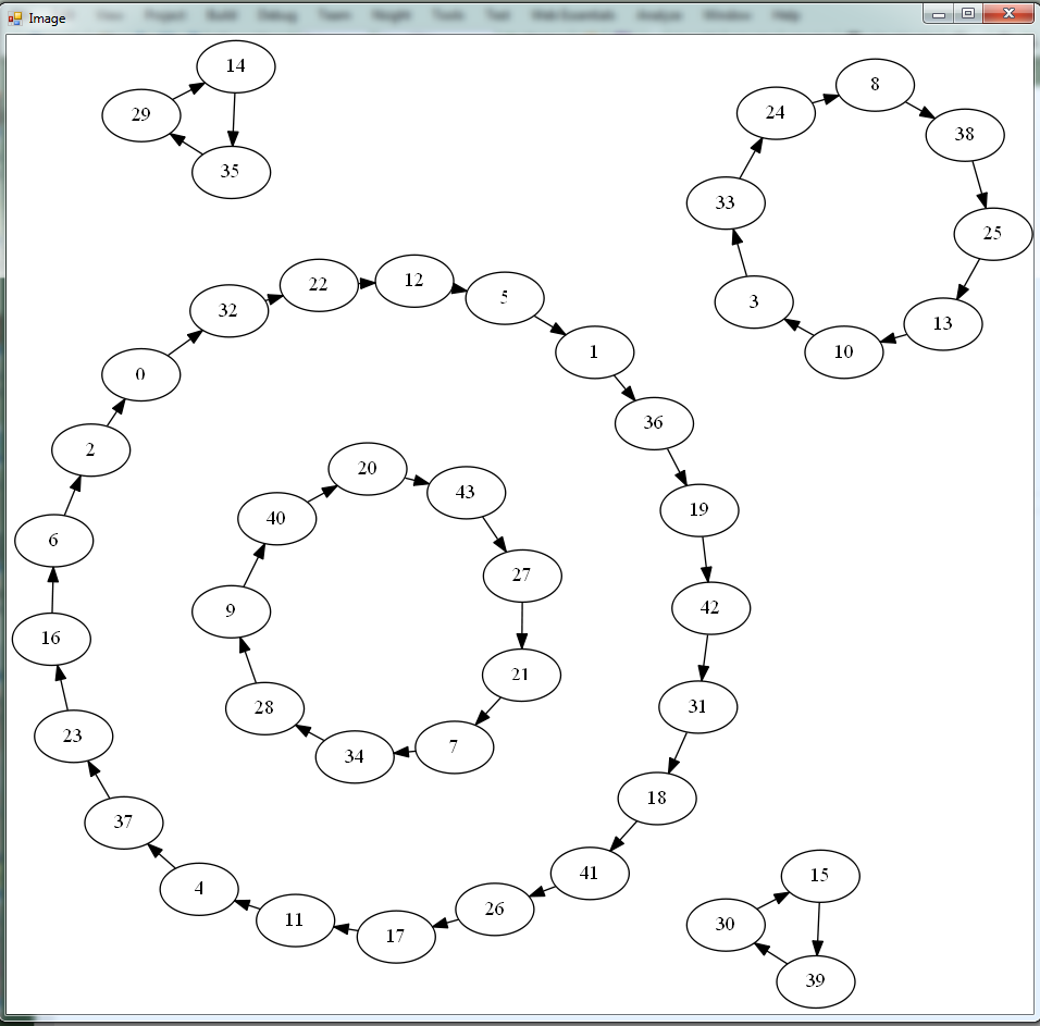
2. At this point, if we are lucky, we have the representation of an Euler cycle as edges of the graph. We just need to walk the array we have “backwards”, seeding the final list of edges with edge 0, constructing the list recursively like so: predecessors.[List.head result] :: result. Alternatively, we may generate a graph out of the result and reverse it. (directions of the arrows need to be reversed since this is a predecessor graph. Euler cycles of the graph, where all directions are reversed are the same as those of the original one, reversed.)

In case we aren’t lucky, we consider our predecessor array to be a graph, where each edge of the original graph becomes a vertex and identify partitions of the graph:

This is the weak point of the algorithm. Partitioning a graph is, in general, a hard problem (NP-complete, to be precise), however, in this case, due to a very simple structure of the predecessor graph, the complexity is linear in the number of edges of the original graph: O(|E|).

let partitionLinear (end' : int [])=
    let allVertices = HashSet<int>(end')
    let colors = Array.create end'.Length -1
    let mutable color = 0

    while allVertices.Count > 0 do
        let mutable v = allVertices.First()
        while colors.[v] < 0 do
            allVertices.Remove v |> ignore
            colors.[v] <- color
            v <- end'.[v]
        color <- color + 1
    colors, color

So, now the goal is to join all the circles above into one circle, this is done in the crucial step 3

3. We further collapse the graph based on partitioning. Now, each partition becomes a vertex of the new graph. Edges of this new “circuit graph” are vertices of the original graph, such that each edge represents a vertex two partitions have in common.

This is the only part of the algorithm where the GPU is used and is very effective. Incidentally, I took the code almost verbatim from the original thesis, however, the author for some reason preferred not to implement this step on the GPU.

The idea is simple: we loop over the original graph vertex-by-vertex and try to figure out whether edges entering this vertex belong to different partitions (have different colors in the terminology of the code above). Each vertex is processed in a CUDA kernel:

let gcGraph, links, validity = generateCircuitGraph gr.RowIndex partition maxPartition
gcGraph.Visualize()

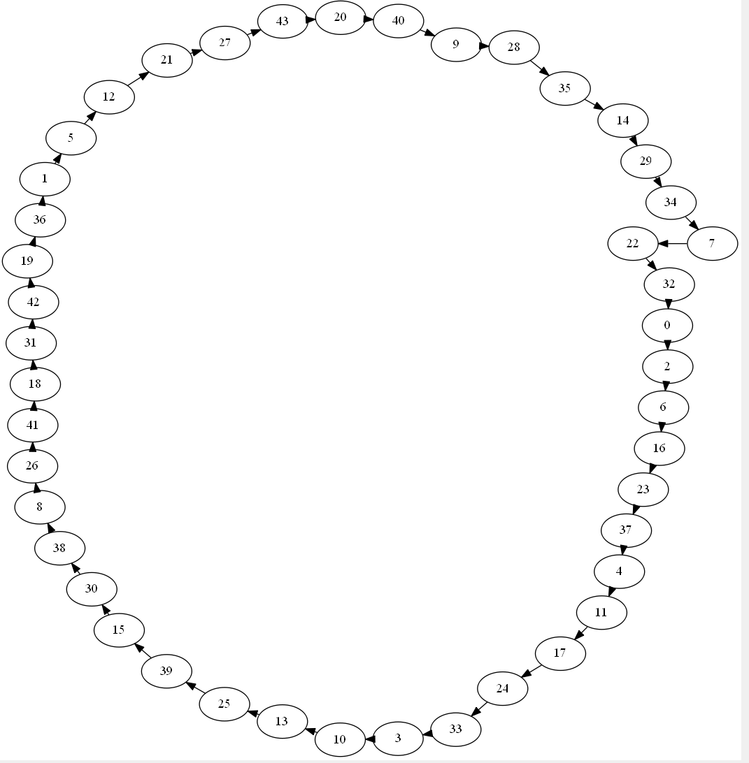
4. This graph is greatly over-determined: we don’t need ALL vertices that partitions have in common (represented by edges here). Also, it’s important to note that this graph is not directed: if partition 0 has a vertex in common with partition 1, then this is the same vertex partition 1 has in common with partition 0. In our implementation this un-directionality is reflected by over-directionality: every edge is repeated as All we actually need is a spanning tree of this graph:

gcGraph.Visualize(spanningTree=true)

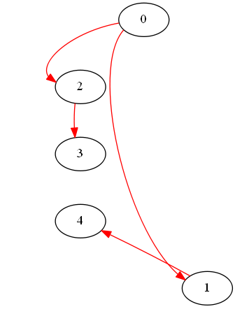
Alright, this is much better – ignore directions. The output of step 3 gives us vertices of the original graph where our partitions intersect. We now need to swap edges of our original predecessor array around these vertices, so that each partition is not closed off on itself, but merges with its neighbor (it’s but a small correction to our original predecessor walk). We do this one-by-one, so partition 0 merges first with 1, then with 2. And 2 – with 3. And 1 with 4.

let fixedPredecessors = fixPredecessors gcGraph links edgePredecessors validity
let finalGraph = StrGraph.FromVectorOfInts fixedPredecessors
finalGraph.Reverse.Visualize()

And it’s a beautiful circle, we are done!

Why not Break out That Cognac?

let N = 1024 * 1024
let i = 1

let gr = StrGraph.GenerateEulerGraphAlt(N * i, 3 * i * N)
let eulerCycle = findEulerTimed gr

Euler graph: vertices - 1,048,575.00, edges - 3,145,727.00
1. Predecessors computed in 00:00:00.3479258
2. Partitioned linear graph in 00:02:48.3658898
Partitions of LG: 45514
# of partitions: 45514 (CPU generation of CG)
3. Circuit graph generated in 00:00:34.1632645
4. Swips implemented in 00:00:00.1707746
GPU: Euler cycle generated in 00:03:23.0505569

This is not very impressive. What’s happening? Unfortunately graph structure holds the key together with the HashSet implementation.

The deeper the graph the better it will fare in the new algorithm. The bottleneck is the partitioning stage. Even though its complexity is theoretically O(|E|), I am using a HashSet to restart partitioning when needed and that presents a problem, as accessing it is not always O(1)!

The methods for Euler graph generation are implemented as GenerateEulerGraph and GenerateEulerGraphAlt. The first one “pleases the code”, and generates graphs that are very deep even when the number of edges is large. Usually I get less than 10 partitions, which means that every time I generate predecessors, I’m pretty much guaranteed to be “almost there” as far as finding a cycle. The second method tends to generate very shallow graphs, as the example above shows: I got a fairly large number of partitions while the number of edges is only around 3 million. So while the rest of the algorithm performance is pretty descent, computing partitions just kills the whole thing.

Store the cognac for another time.